Getting Started with Athlytics
Athlytics Package
2026-01-18
Source:vignettes/athlytics_introduction.Rmd
athlytics_introduction.RmdWelcome to Athlytics
This tutorial will guide you through a complete workflow—from loading your Strava data to generating training analytics. By the end, you’ll understand how to use all core features of Athlytics for longitudinal exercise physiology analysis.
What You’ll Learn:
- How to load and explore your Strava export data
- Calculate and interpret training load metrics (ACWR)
- Analyze aerobic fitness trends (Efficiency Factor)
- Quantify cardiovascular drift (Decoupling)
- Track personal bests and performance progression
- Export results for further analysis
Time Required: 30-60 minutes
Prerequisites
Installation
For installation instructions, see the README. The quick version:
# CRAN (stable)
install.packages("Athlytics")

# GitHub (latest features)
remotes::install_github("HzaCode/Athlytics")
Your Strava Data Export
You’ll need a Strava data export ZIP file. If you haven’t exported your data yet, start from Strava and follow the steps in the README Quick Start.
Quick Summary: 1. Go to Strava Settings → My Account
→ Download or Delete Your Account 2. Request “Download” (NOT delete!) 3.
Wait for email with download link 4. Download the ZIP file (e.g.,
export_12345678.zip) 5. Don’t unzip it —
Athlytics reads ZIP files directly
Loading Your Data
Understanding the Data Structure
Let’s explore what we just loaded:
# How many activities do you have?
nrow(activities)
# Example output: [1] 847

# What sports are in your data?
table(activities$type)
# Example output:
#   Ride  Run  Swim
#    312  498    37

# Date range
range(activities$date, na.rm = TRUE)
# Example output: [1] "2018-01-05" "2024-12-20"

# Key columns in the dataset
names(activities)
Important Columns:
-
activity_id— Unique identifier -
date— Activity date -
sport— Activity type (Run, Ride, Swim, etc.) -
distance_km— Distance in kilometers -
duration_mins— Duration in minutes -
avg_hr— Average heart rate (if recorded) -
max_hr— Maximum heart rate -
avg_pace_min_km— Average pace for running -
avg_speed_kmh— Average speed -
avg_power— Average power for cycling (if available) -
elevation_gain— Total elevation gain (meters) -
best_efforts— Personal best times at various distances
Data Quality Checks
Before analysis, it’s good practice to check your data:
# Summary statistics
summary(activities %>% select(distance_km, duration_mins, avg_hr))

# Check for missing heart rate data
sum(!is.na(activities$avg_hr)) / nrow(activities) * 100
# Shows % of activities with HR data

# Activities without HR data
activities %>%
  filter(is.na(avg_hr)) %>%
  count(sport)
Pro Tip: Many Athlytics functions require heart rate
data. Filter for !is.na(avg_hr) when calculating EF or
decoupling.
Filtering Your Data
For focused analysis, you’ll often want to filter by sport or date:
# Only running activities
runs <- activities %>%
  filter(sport == "Run")

# Recent activities (last 6 months)
recent <- activities %>%
  filter(date >= Sys.Date() - 180)

# Runs with heart rate data from 2024
runs_2024_hr <- activities %>%
  filter(
    sport == "Run",
    !is.na(avg_hr),
    lubridate::year(date) == 2024
  )

# Long runs only (> 15 km)
long_runs <- activities %>%
  filter(sport == "Run", distance_km > 15)
Core Analyses
Now let’s dive into the main analytical features. Each metric provides different insights into your training and physiology.
1. Training Load (ACWR)
What is ACWR?
The Acute:Chronic Workload Ratio (ACWR) compares your recent training (acute load, typically 7 days) to your long-term baseline (chronic load, typically 28 days). It’s used to identify injury risk periods.
Risk Zones:
- < 0.8 — Undertraining (fitness may decline)
- 0.8-1.3 — “Sweet spot” (optimal adaptation zone)
- 1.3-1.5 — Moderate risk (load increasing rapidly)
- > 1.5 — High risk (excessive load spike, injury risk)
Basic ACWR Calculation
# Calculate ACWR for all running activities
acwr_data <- calculate_acwr(
  activities_data = runs,
  activity_type = "Run", # Filter by sport
  load_metric = "duration_mins", # Can also be "distance_km" or "hrss"
  acute_period = 7, # 7-day rolling average
  chronic_period = 28 # 28-day rolling average
)

# View results
head(acwr_data)
Output Columns:
-
date— Date -
daily_load— Training load for that day (sum of duration/distance) -
atl— Acute Training Load (7-day rolling average) -
ctl— Chronic Training Load (28-day rolling average) -
acwr_smooth— The ACWR ratio (ATL / CTL)
Visualizing ACWR
# Basic plot
plot_acwr(acwr_data)

# With risk zones highlighted (recommended)
plot_acwr(acwr_data, highlight_zones = TRUE)
Demo with Sample Data:
# Load built-in sample data
data("sample_acwr", package = "Athlytics")

# Plot ACWR with risk zones
plot_acwr(sample_acwr, highlight_zones = TRUE)
#> Generating plot...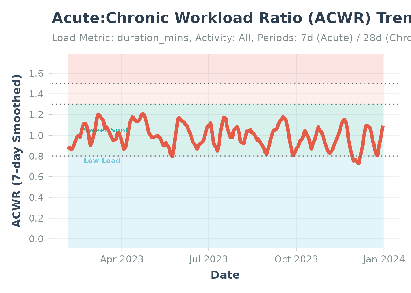
ACWR visualization using sample data
Interpreting Your ACWR
What to look for:
- Gradual increases = Good progressive overload
- Sharp spikes above 1.5 = Warning signs, consider recovery
- Extended periods < 0.8 = May need to increase training volume
- Stable values in 0.8-1.3 = Optimal training stimulus
Practical Example:
Choosing Load Metrics
Different load metrics for different goals:
-
duration_mins— Simple, works for all sports, good for general monitoring -
distance_km— Better for distance-focused training (marathon prep) -
hrss— Most accurate for physiological load (requires HR data)
# Calculate using HRSS (heart rate stress score)
acwr_hrss <- calculate_acwr(
  activities_data = runs,
  load_metric = "hrss" # Automatically calculated if avg_hr available
)
2. Efficiency Factor (EF)
What is EF?
Efficiency Factor measures how much output (speed/power) you generate per unit of input (heart rate). It’s a key indicator of aerobic fitness improvements.
Metrics:
- Pace/HR (running) — Speed per heartbeat: Higher = better aerobic fitness
- Power/HR (cycling) — Watts per heartbeat: Higher = better aerobic fitness
What Changes Mean:
- Increasing EF = Aerobic fitness improving (doing more work at same HR)
- Stable EF = Maintaining current fitness
- Decreasing EF = Fatigue, overtraining, or fitness loss
Calculate EF
# For running (Pace/HR)
ef_runs <- calculate_ef(
  activities_data = runs,
  activity_type = "Run",
  ef_metric = "pace_hr" # Pace divided by HR
)

# For cycling (Power/HR)
rides <- activities %>% filter(sport == "Ride")
ef_cycling <- calculate_ef(
  activities_data = rides,
  activity_type = "Ride",
  ef_metric = "power_hr" # Power divided by HR
)

# View results
head(ef_runs)
Output Columns:
-
date— Activity date -
ef_value— Efficiency Factor value -
avg_hr— Average heart rate -
avg_pace_min_km(oravg_power) — Output metric
Visualizing EF Trends
# Basic plot
plot_ef(ef_runs)

# With smoothing line to see trend (recommended)
plot_ef(ef_runs, add_trend_line = TRUE)
Demo with Sample Data:
# Load built-in sample data
data("sample_ef", package = "Athlytics")

# Plot EF with trend line
plot_ef(sample_ef, add_trend_line = TRUE)
#> Generating plot...
#> `geom_smooth()` using formula = 'y ~ x'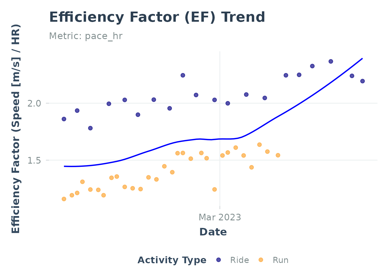
Efficiency Factor trend using sample data
Interpreting EF
Best Practices:
- Track trends over weeks/months, not day-to-day fluctuations
- Use steady-state efforts only — Interval workouts will skew results
- Consider external factors — Heat, altitude, fatigue affect EF
Practical Analysis:
# Calculate monthly average EF
library(lubridate)

ef_monthly <- ef_runs %>%
  mutate(month = floor_date(date, "month")) %>%
  group_by(month) %>%
  summarise(
    mean_ef = mean(ef_value, na.rm = TRUE),
    n_activities = n()
  ) %>%
  arrange(desc(month))

print(ef_monthly)

# Compare first vs last 3 months
recent_ef <- ef_runs %>%
  filter(date >= Sys.Date() - 90) %>%
  pull(ef_value)
baseline_ef <- ef_runs %>%
  filter(date < Sys.Date() - 90, date >= Sys.Date() - 180) %>%
  pull(ef_value)

cat(sprintf(
  "Recent EF: %.2f\nBaseline EF: %.2f\nChange: %.1f%%\n",
  mean(recent_ef, na.rm = TRUE),
  mean(baseline_ef, na.rm = TRUE),
  (mean(recent_ef, na.rm = TRUE) / mean(baseline_ef, na.rm = TRUE) - 1) * 100
))
3. Cardiovascular Decoupling
What is Decoupling?
Decoupling quantifies cardiovascular drift—the phenomenon where heart rate gradually rises during prolonged efforts even if pace/power remains constant. Low decoupling indicates good aerobic endurance.
How It Works:
The function compares efficiency (pace/HR or power/HR) between the first half and second half of an activity:
Positive values = efficiency decline in second half (HR drift); <5% commonly used as reference threshold, requires interpretation in context of steady-state and environmental conditions.
Interpretation:
- < 5% — Excellent aerobic base, well-adapted
- 5-10% — Acceptable, some drift but manageable
- > 10% — Significant drift (fatigue, heat, insufficient base fitness)
Calculate Decoupling
# For running
decoupling_runs <- calculate_decoupling(
  activities_data = runs,
  activity_type = "Run",
  decouple_metric = "pace_hr",
  min_duration_mins = 60 # Only analyze runs ≥ 60 minutes
)

# For cycling
decoupling_rides <- calculate_decoupling(
  activities_data = rides,
  activity_type = "Ride",
  decouple_metric = "power_hr",
  min_duration_mins = 90 # Longer threshold for cycling
)

# View results
head(decoupling_runs)
Output Columns:
-
date— Activity date -
first_half_ratio— EF in first half -
second_half_ratio— EF in second half -
decoupling_pct— Percentage drift
Visualizing Decoupling
# Basic plot
plot_decoupling(decoupling_runs)

# With metric specification
plot_decoupling(decoupling_runs, decouple_metric = "pace_hr")
Demo with Sample Data:
# Load built-in sample data
data("sample_decoupling", package = "Athlytics")

# Plot decoupling trend (use decoupling_df parameter)
plot_decoupling(decoupling_df = sample_decoupling)
#> Generating plot...
#> `geom_smooth()` using formula = 'y ~ x'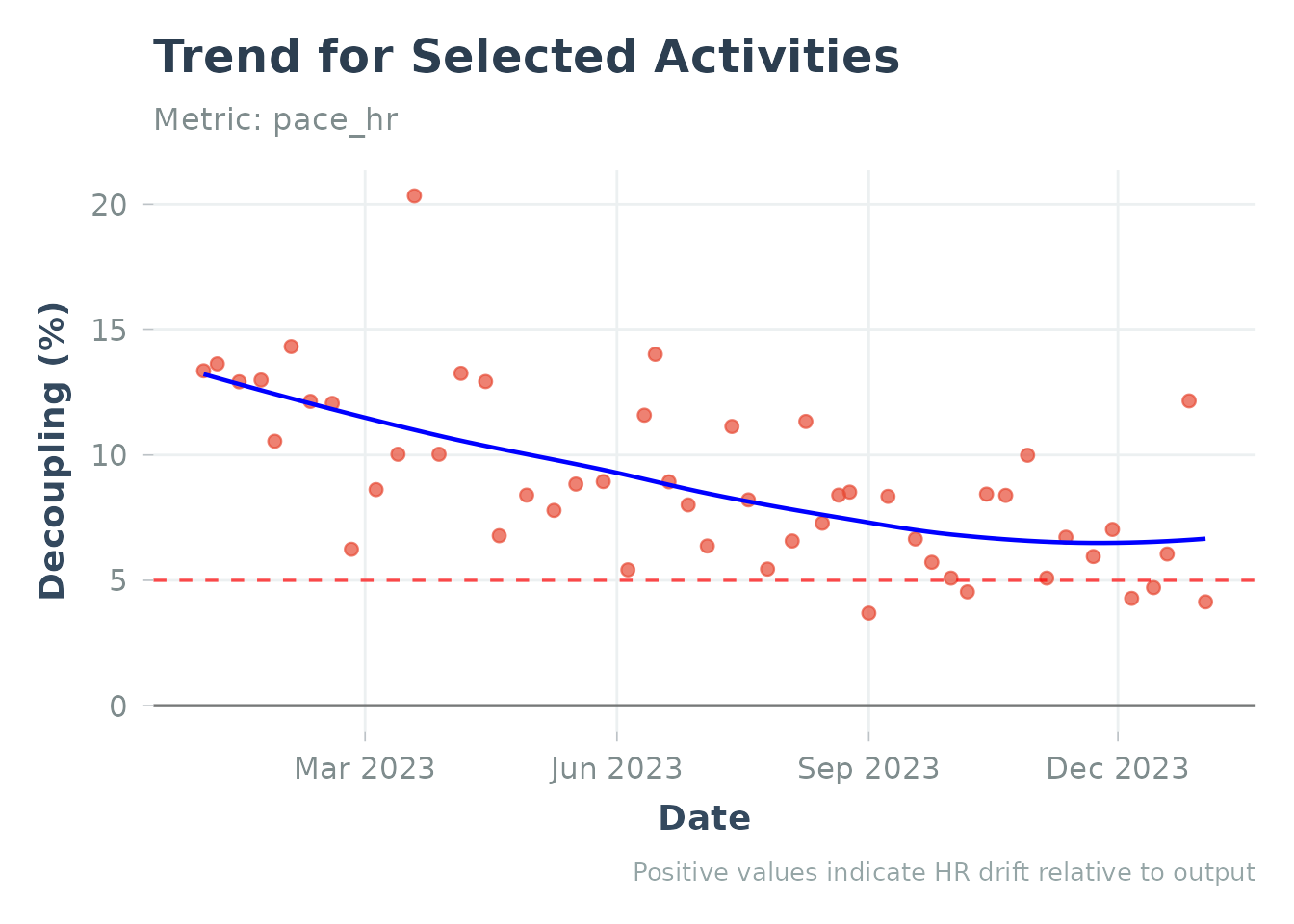
Cardiovascular decoupling using sample data
Practical Applications
1. Assess Aerobic Base:
# Recent decoupling average
recent_decouple <- decoupling_runs %>%
  filter(date >= Sys.Date() - 60) %>%
  summarise(avg_decouple = mean(decoupling_pct, na.rm = TRUE))

if (recent_decouple$avg_decouple < 5) {
  cat("Excellent aerobic base! Ready for higher intensity.\n")
} else if (recent_decouple$avg_decouple < 10) {
  cat("Good base, continue building aerobic foundation.\n")
} else {
  cat("High decoupling—focus on more easy, long runs.\n")
}
2. Monitor Training Block Progress:
# Compare decoupling over time
library(ggplot2)

decoupling_runs %>%
  ggplot(aes(x = date, y = decoupling_pct)) +
  geom_point(alpha = 0.6) +
  geom_smooth(method = "loess", se = TRUE) +
  geom_hline(yintercept = 5, linetype = "dashed", color = "green") +
  geom_hline(yintercept = 10, linetype = "dashed", color = "orange") +
  labs(
    title = "Decoupling Trend Over Time",
    subtitle = "Lower values = better aerobic endurance",
    x = "Date", y = "Decoupling (%)"
  ) +
  theme_minimal()
Important Note: Decoupling is highly affected by environmental conditions (heat, humidity) and cumulative fatigue. Always interpret in context.
4. Personal Bests (PBs)
Track your best performances at standard distances over time.
Calculate PBs
# Extract personal bests
pbs <- calculate_pbs(
  activities_data = runs,
  activity_type = "Run"
)

# View all PRs
print(pbs)
Supported Distances:
- 400m, 800m, 1km, 1 mile
- 5km, 10km
- Half marathon, Marathon
Visualize PB Progression
# Plot PR progression
plot_pbs(pbs)

# Filter to specific distance
pbs_5k <- pbs %>% filter(distance == "5k")
print(pbs_5k)
Demo with Sample Data:
# Load built-in sample data
data("sample_pbs", package = "Athlytics")

# Plot PB progression (use pbs_df parameter)
plot_pbs(pbs_df = sample_pbs)
#> Generating plot...
#> `geom_smooth()` using formula = 'y ~ x'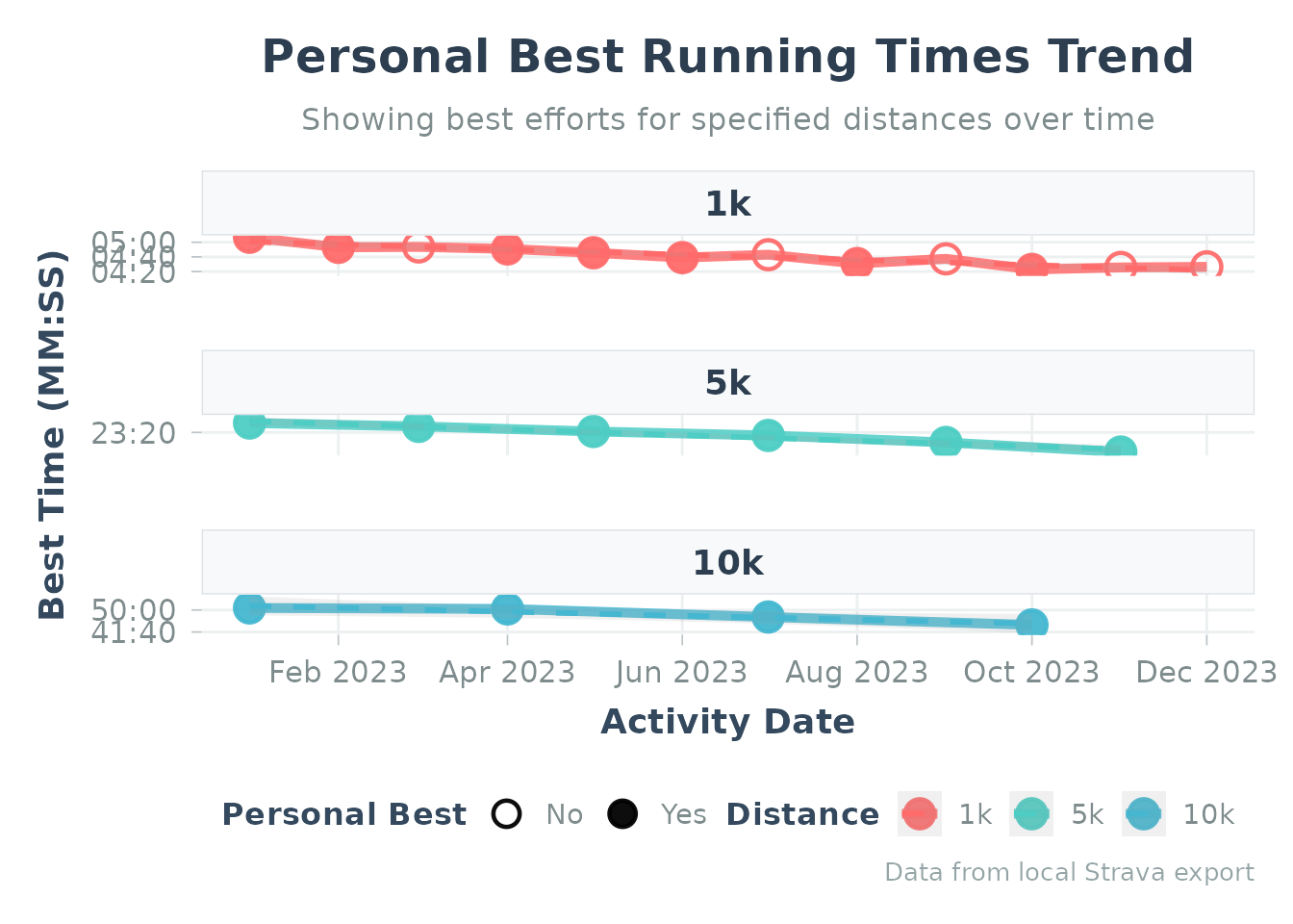
Personal bests progression using sample data
5. Load Exposure Analysis
Visualize your training state in 2D space: acute load vs chronic load.
Calculate and Plot Exposure
# Calculate exposure
exposure <- calculate_exposure(
  activities_data = runs,
  activity_type = "Run",
  load_metric = "duration_mins"
)

# Plot with risk zones
plot_exposure(exposure, highlight_zones = TRUE)
Demo with Sample Data:
# Load built-in sample data
data("sample_exposure", package = "Athlytics")

# Plot exposure (use exposure_df parameter)
plot_exposure(exposure_df = sample_exposure, activity_type = "Run")
#> Generating plot...
#> Warning: Removed 27 rows containing missing values or values outside the scale range
#> (`geom_point()`).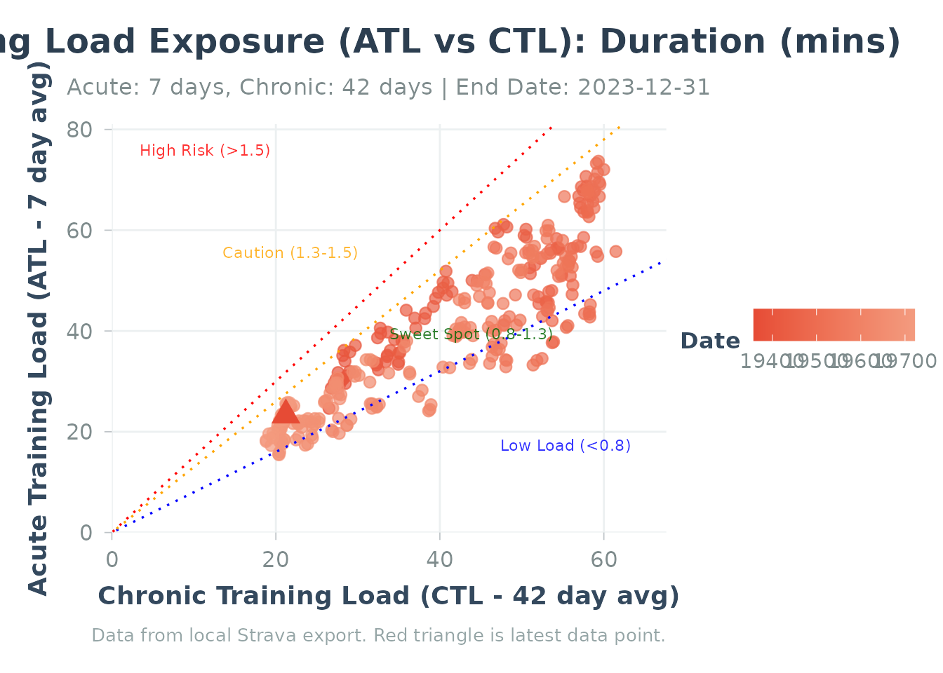
Load exposure analysis using sample data
Interpretation:
- Points above diagonal = Acute > chronic (ramping up training)
- Points on diagonal = Balanced state
- Points below diagonal = Tapering or recovery
- Red zone = High ACWR, injury risk
Complete Workflow Example
Here’s a realistic, end-to-end analysis workflow:
library(Athlytics)
library(dplyr)
library(ggplot2)

# ---- 1. Load and Filter Data ----
activities <- load_local_activities("my_strava_export.zip")

# Focus on running activities with HR data
runs <- activities %>%
  filter(sport == "Run", !is.na(avg_hr))

cat(sprintf("Loaded %d running activities with HR data\n", nrow(runs)))

# ---- 2. Training Load Monitoring ----
acwr_data <- calculate_acwr(
  activities_data = runs,
  load_metric = "duration_mins"
)

# Check current training status
current_acwr <- acwr_data %>%
  filter(date >= Sys.Date() - 30) %>%
  tail(1) %>%
  pull(acwr_smooth)

cat(sprintf("Current ACWR: %.2f\n", current_acwr))

# Visualize
p1 <- plot_acwr(acwr_data, highlight_zones = TRUE) +
  labs(title = "6-Month Training Load Progression")
print(p1)

# ---- 3. Aerobic Fitness Tracking ----
ef_data <- calculate_ef(
  activities_data = runs,
  ef_metric = "pace_hr"
)

# Calculate fitness trend
ef_trend <- ef_data %>%
  mutate(month = lubridate::floor_date(date, "month")) %>%
  group_by(month) %>%
  summarise(mean_ef = mean(ef_value, na.rm = TRUE))

p2 <- plot_ef(ef_data, add_trend_line = TRUE) +
  labs(title = "Aerobic Efficiency Trend")
print(p2)

# ---- 4. Endurance Assessment ----
# Only for long runs (> 60 min)
decoupling_data <- calculate_decoupling(
  activities_data = runs,
  min_duration_mins = 60
)

avg_decouple <- mean(decoupling_data$decoupling_pct, na.rm = TRUE)
cat(sprintf(
  "Average decoupling: %.1f%% (%s aerobic base)\n",
  avg_decouple,
  ifelse(avg_decouple < 5, "excellent",
    ifelse(avg_decouple < 10, "good", "needs work")
  )
))

p3 <- plot_decoupling(decoupling_data) +
  labs(title = "Cardiovascular Drift in Long Runs")
print(p3)

# ---- 5. Export Results ----
# Save plots
ggsave("acwr_analysis.png", plot = p1, width = 10, height = 6, dpi = 300)
ggsave("ef_trend.png", plot = p2, width = 10, height = 6, dpi = 300)
ggsave("decoupling.png", plot = p3, width = 10, height = 6, dpi = 300)

# Export data for further analysis
write.csv(acwr_data, "acwr_results.csv", row.names = FALSE)
write.csv(ef_data, "ef_results.csv", row.names = FALSE)
write.csv(decoupling_data, "decoupling_results.csv", row.names = FALSE)

cat("\nAnalysis complete! Results saved.\n")
Troubleshooting
Common Issues
“No data returned” or empty results
Causes: - Activity type filter doesn’t match your data - Required metrics (e.g., HR) are missing - Date range has no activities
Solutions:
# Check activity types in your data
table(activities$type)

# Check for HR data availability
sum(!is.na(activities$average_heartrate))

# Verify date range
range(activities$date, na.rm = TRUE)

# Try without filtering first
test <- calculate_acwr(activities_data = activities, activity_type = NULL)
“Not enough data for chronic period”
ACWR requires at least 28 days of data. Check your date range:
# How much data do you have?
date_span <- as.numeric(max(activities$date) - min(activities$date))
cat(sprintf("Your data spans %d days\n", date_span))

# If < 28 days, you need more data or use shorter periods
“NA values in output”
Some activities may lack required metrics (HR, power, etc.):
# Filter before calculating
runs_with_hr <- runs %>% filter(!is.na(avg_hr))
ef_data <- calculate_ef(runs_with_hr, ef_metric = "pace_hr")Getting Help
-
Function documentation:
?calculate_acwr,?plot_ef, etc. - GitHub Issues: Report bugs
-
Package vignettes:
browseVignettes("Athlytics")
Next Steps
Congratulations! You now know how to use all core features of Athlytics.
Advanced Features
Ready to go deeper? Check out:
- Advanced Features Tutorial — EWMA-based ACWR with confidence intervals, quality control, and cohort analysis
- Function Reference — Complete documentation of all functions
For Researchers
If you’re using Athlytics for research:
- Cohort Studies: See calculate_cohort_reference() for multi-athlete percentile comparisons
- Data Quality: Use flag_quality() for stream data quality control
- Statistical Analysis: All functions return tidy data frames ready for lme4, survival analysis, etc.
Session Info
sessionInfo()
#> R version 4.5.2 (2025-10-31)
#> Platform: x86_64-pc-linux-gnu
#> Running under: Ubuntu 24.04.3 LTS
#>
#> Matrix products: default
#> BLAS:   /usr/lib/x86_64-linux-gnu/openblas-pthread/libblas.so.3
#> LAPACK: /usr/lib/x86_64-linux-gnu/openblas-pthread/libopenblasp-r0.3.26.so;  LAPACK version 3.12.0
#>
#> locale:
#>  [1] LC_CTYPE=C.UTF-8       LC_NUMERIC=C           LC_TIME=C.UTF-8
#>  [4] LC_COLLATE=C.UTF-8     LC_MONETARY=C.UTF-8    LC_MESSAGES=C.UTF-8
#>  [7] LC_PAPER=C.UTF-8       LC_NAME=C              LC_ADDRESS=C
#> [10] LC_TELEPHONE=C         LC_MEASUREMENT=C.UTF-8 LC_IDENTIFICATION=C
#>
#> time zone: UTC
#> tzcode source: system (glibc)
#>
#> attached base packages:
#> [1] stats     graphics  grDevices utils     datasets  methods   base
#>
#> other attached packages:
#> [1] ggplot2_4.0.1   Athlytics_1.0.2
#>
#> loaded via a namespace (and not attached):
#>  [1] sass_0.4.10        generics_0.1.4     tidyr_1.3.2        lattice_0.22-7
#>  [5] hms_1.1.4          digest_0.6.39      magrittr_2.0.4     evaluate_1.0.5
#>  [9] grid_4.5.2         timechange_0.3.0   RColorBrewer_1.1-3 fastmap_1.2.0
#> [13] jsonlite_2.0.0     Matrix_1.7-4       mgcv_1.9-3         purrr_1.2.1
#> [17] viridisLite_0.4.2  scales_1.4.0       textshaping_1.0.4  jquerylib_0.1.4
#> [21] cli_3.6.5          rlang_1.1.7        splines_4.5.2      withr_3.0.2
#> [25] cachem_1.1.0       yaml_2.3.12        otel_0.2.0         tools_4.5.2
#> [29] tzdb_0.5.0         dplyr_1.1.4        vctrs_0.7.0        R6_2.6.1
#> [33] zoo_1.8-15         lifecycle_1.0.5    lubridate_1.9.4    fs_1.6.6
#> [37] htmlwidgets_1.6.4  ragg_1.5.0         pkgconfig_2.0.3    desc_1.4.3
#> [41] pkgdown_2.2.0      pillar_1.11.1      bslib_0.9.0        gtable_0.3.6
#> [45] glue_1.8.0         systemfonts_1.3.1  xfun_0.55          tibble_3.3.1
#> [49] tidyselect_1.2.1   knitr_1.51         farver_2.1.2       htmltools_0.5.9
#> [53] nlme_3.1-168       rmarkdown_2.30     labeling_0.4.3     readr_2.1.6
#> [57] compiler_4.5.2     S7_0.2.1