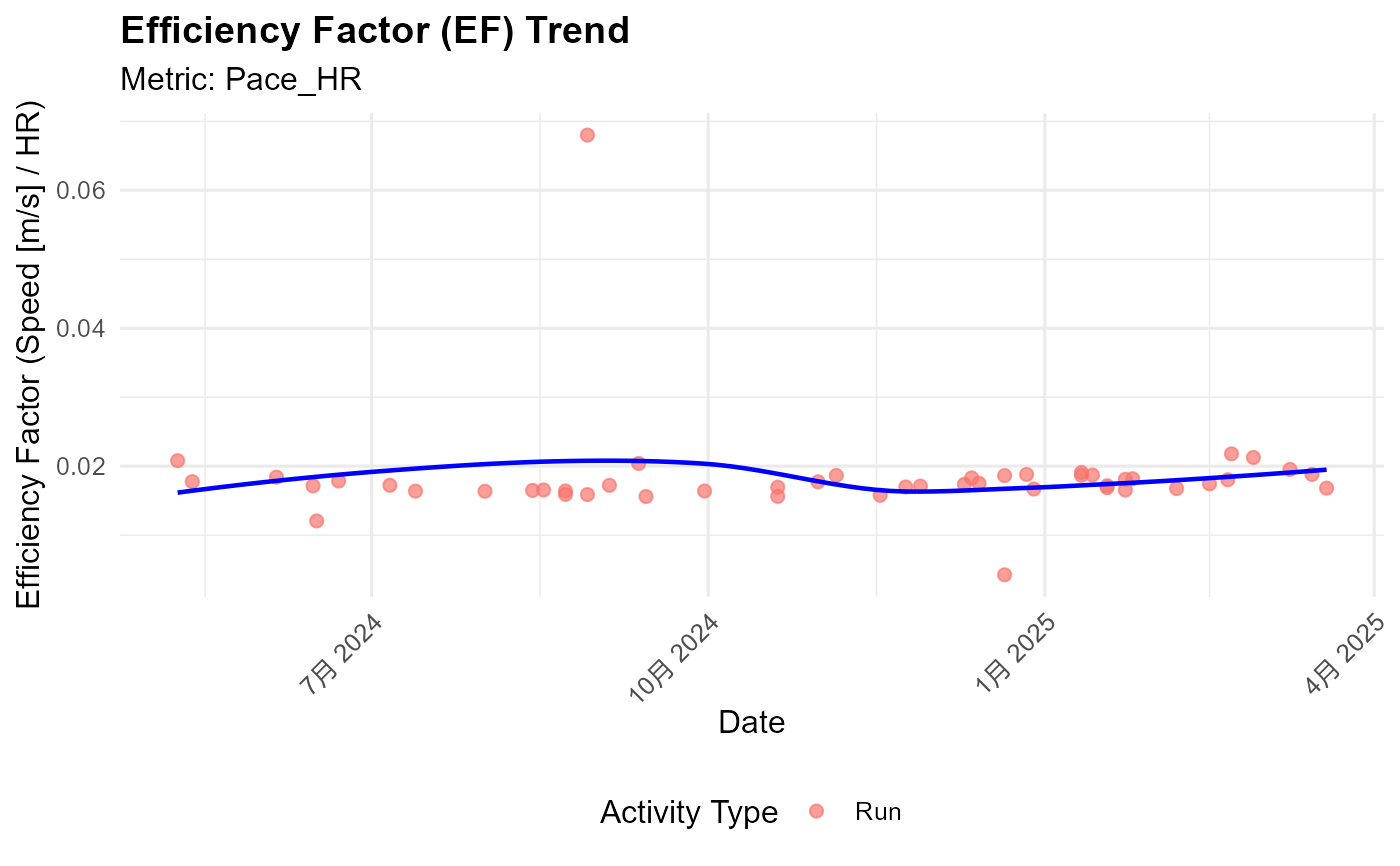
Plot Efficiency Factor (EF) Trend — plot

Visualizes the trend of Efficiency Factor (EF) over time.

Usage

plot_ef(
  data,
  activity_type = c("Run", "Ride"),
  ef_metric = c("pace_hr", "power_hr"),
  start_date = NULL,
  end_date = NULL,
  min_duration_mins = 20,
  add_trend_line = TRUE,
  smoothing_method = "loess",
  ef_df = NULL,
  group_var = NULL,
  group_colors = NULL
)

Arguments

data: Recommended: Pass pre-calculated data via ef_df (local export preferred). A data frame from calculate_ef() or activities data from load_local_activities().
activity_type: Type(s) of activities to analyze (e.g., "Run", "Ride").
ef_metric: Metric to calculate: "pace_hr" (Speed/HR) or "power_hr" (Power/HR).
start_date: Optional. Analysis start date (YYYY-MM-DD string or Date). Defaults to ~1 year ago.
end_date: Optional. Analysis end date (YYYY-MM-DD string or Date). Defaults to today.
min_duration_mins: Minimum activity duration (minutes) to include. Default 20.
add_trend_line: Add a smoothed trend line (geom_smooth)? Default TRUE.
smoothing_method: Smoothing method for trend line (e.g., "loess", "lm"). Default "loess".
ef_df: Recommended. A pre-calculated data frame from calculate_ef(). When provided, analysis uses local data only (no API calls).
group_var: Optional. Column name for grouping/faceting (e.g., "athlete_id").
group_colors: Optional. Named vector of colors for groups.

Value

A ggplot object showing the EF trend.

Details

Plots the Efficiency Factor (EF) trend over time. Recommended workflow: Use local data via ef_df.

Plots EF (output/HR based on activity averages). An upward trend often indicates improved aerobic fitness. Points colored by activity type. Best practice: Use load_local_activities() + calculate_ef() + this function.

Examples

# Example using pre-calculated sample data
data("athlytics_sample_ef", package = "Athlytics")
p <- plot_ef(athlytics_sample_ef)
#> Generating plot...
print(p)
#> `geom_smooth()` using formula = 'y ~ x'


if (FALSE) { # \dontrun{
# Example using local Strava export data
activities <- load_local_activities("strava_export_data/activities.csv")

# Plot Pace/HR EF trend for Runs (last 6 months)
plot_ef(data = activities,
        activity_type = "Run",
        ef_metric = "pace_hr",
        start_date = Sys.Date() - months(6))

# Plot Power/HR EF trend for Rides
plot_ef(data = activities,
        activity_type = "Ride",
        ef_metric = "power_hr")

# Plot Pace/HR EF trend for multiple Run types (no trend line)
plot_ef(data = activities,
        activity_type = c("Run", "VirtualRun"),
        ef_metric = "pace_hr",
        add_trend_line = FALSE)
} # }