Plot ACWR Trend

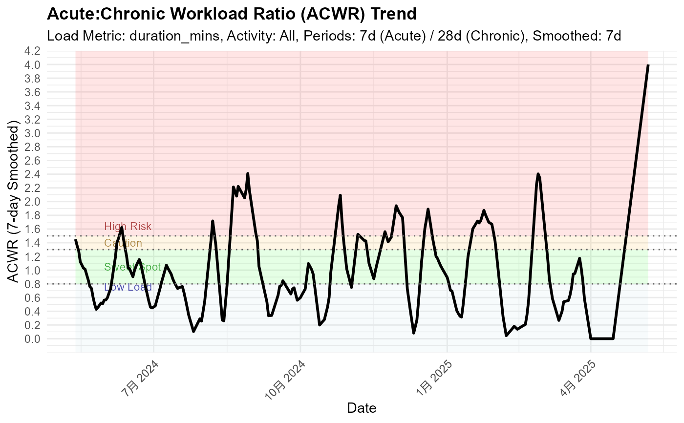
Visualizes the Acute:Chronic Workload Ratio (ACWR) trend over time.

Usage

plot_acwr(
  data,
  activity_type = NULL,
  load_metric = "duration_mins",
  acute_period = 7,
  chronic_period = 28,
  start_date = NULL,
  end_date = NULL,
  user_ftp = NULL,
  user_max_hr = NULL,
  user_resting_hr = NULL,
  smoothing_period = 7,
  highlight_zones = TRUE,
  acwr_df = NULL,
  group_var = NULL,
  group_colors = NULL
)

Arguments

data

Recommended: Pass pre-calculated data via acwr_df (local export preferred). A data frame from calculate_acwr() or activities data from load_local_activities().

activity_type

Type(s) of activities to analyze (e.g., "Run", "Ride").

load_metric

Method for calculating daily load (e.g., "duration_mins", "distance_km", "tss", "hrss").

acute_period

Days for the acute load window (e.g., 7).

chronic_period

Days for the chronic load window (e.g., 28). Must be greater than acute_period.

start_date

Optional. Analysis start date (YYYY-MM-DD string or Date). Defaults to ~1 year ago.

end_date

Optional. Analysis end date (YYYY-MM-DD string or Date). Defaults to today.

user_ftp

Required if load_metric = "tss" and acwr_df is not provided. Your Functional Threshold Power.

user_max_hr

Required if load_metric = "hrss" and acwr_df is not provided. Your maximum heart rate.

user_resting_hr

Required if load_metric = "hrss" and acwr_df is not provided. Your resting heart rate.

smoothing_period

Days for smoothing the ACWR using a rolling mean (e.g., 7). Default 7.

highlight_zones

Logical, whether to highlight different ACWR zones (e.g., sweet spot, high risk) on the plot. Default TRUE.

acwr_df

Recommended. A pre-calculated data frame from calculate_acwr() or calculate_acwr_ewma(). When provided, analysis uses local data only (no API calls).

group_var

Optional. Column name for grouping/faceting (e.g., "athlete_id").

group_colors

Optional. Named vector of colors for groups.

Value

A ggplot object showing the ACWR trend.

Details

Plots the ACWR trend over time. Best practice: Use load_local_activities() + calculate_acwr() + this function. ACWR is calculated as acute load / chronic load. A ratio of 0.8-1.3 is often considered the "sweet spot".

Examples

# Example using pre-calculated sample data
data("athlytics_sample_acwr", package = "Athlytics")
p <- plot_acwr(athlytics_sample_acwr)
#> Generating plot...
print(p)


if (FALSE) { # \dontrun{
# Example using local Strava export data
activities <- load_local_activities("strava_export_data/activities.csv")

# Plot ACWR trend for Runs (using duration as load metric)
plot_acwr(data = activities,
          activity_type = "Run",
          load_metric = "duration_mins",
          acute_period = 7,
          chronic_period = 28)

# Plot ACWR trend for Rides (using TSS as load metric)
plot_acwr(data = activities,
          activity_type = "Ride",
          load_metric = "tss",
          user_ftp = 280)  # FTP value is required
} # }